Our 2021 Big Data Bowl Submission

data science

sports analytics

Author

Matt Kaye

Published

January 7, 2021

Introduction

Our project aims to measure the ability of defensive backs at performing different aspects of their defensive duties: deterring targets (either by reputation or through good positioning), closing down receivers, and breaking up passes. We do this by fitting four models, two for predicting the probability that a receiver will be targeted on a given play and two for predicting the probability that a pass will be caught, which we then use to aggregate the contributions of defensive backs over the course of the season.

Modeling Framework

We opted to use XGBoost for all of our models. At a high level, we chose a tree booster for its ability to find complex interactions between predictors, something we anticipated would be necessary for this project. Tree boosting also allows for null values to be present, which helped us divvy up credit in the catch probability models (more on this later). Finally, tree boosting is a relatively simple, easy-to-tune algorithm that generally performs extremely well, as was the case for us.

Catch Probability

Our catch probability model has two distinct components: The catch probability at throw time – as in, the chance that the pass is caught at the time the quarterback releases the ball – and the catch probability at arrival time – the chance the pass is caught at the time the ball arrives. These probabilities are distinct since a lot can happen between throw release and throw arrival. First, we will walk through the features that are used in building each model.

For the throw time model (which we will refer to as the “throw” model) and the arrival time model (the “arrival” model), the most important predictors by variable importance were what we expected entering this project: the distance of the receiver to the closest defender, the position of the receiver in the \(y\) direction (i.e. distance from the sideline), the distance of the throw, the position of the football in the \(y\) direction at arrival time (this is mostly catching throws to the sideline and throw aways), the velocity of the throw, the velocity and acceleration of the targeted receiver, and a composite receiver skill metric. For the arrival model, we use many of the same features. However, we do not account for the distance of the defenders to the throw vector – which accounts for the ability to break up a pass mid-flight – because the throw has already arrived.

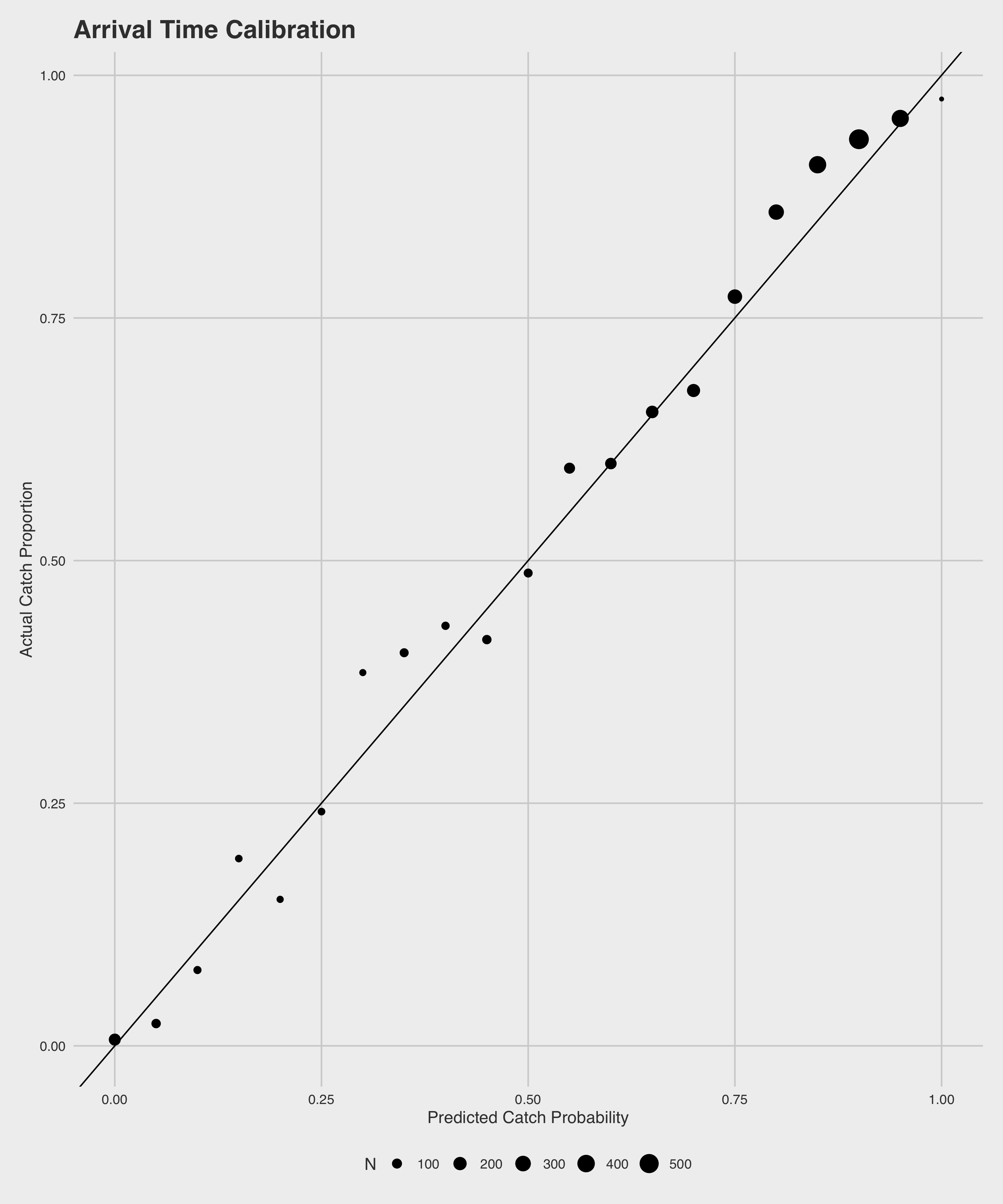
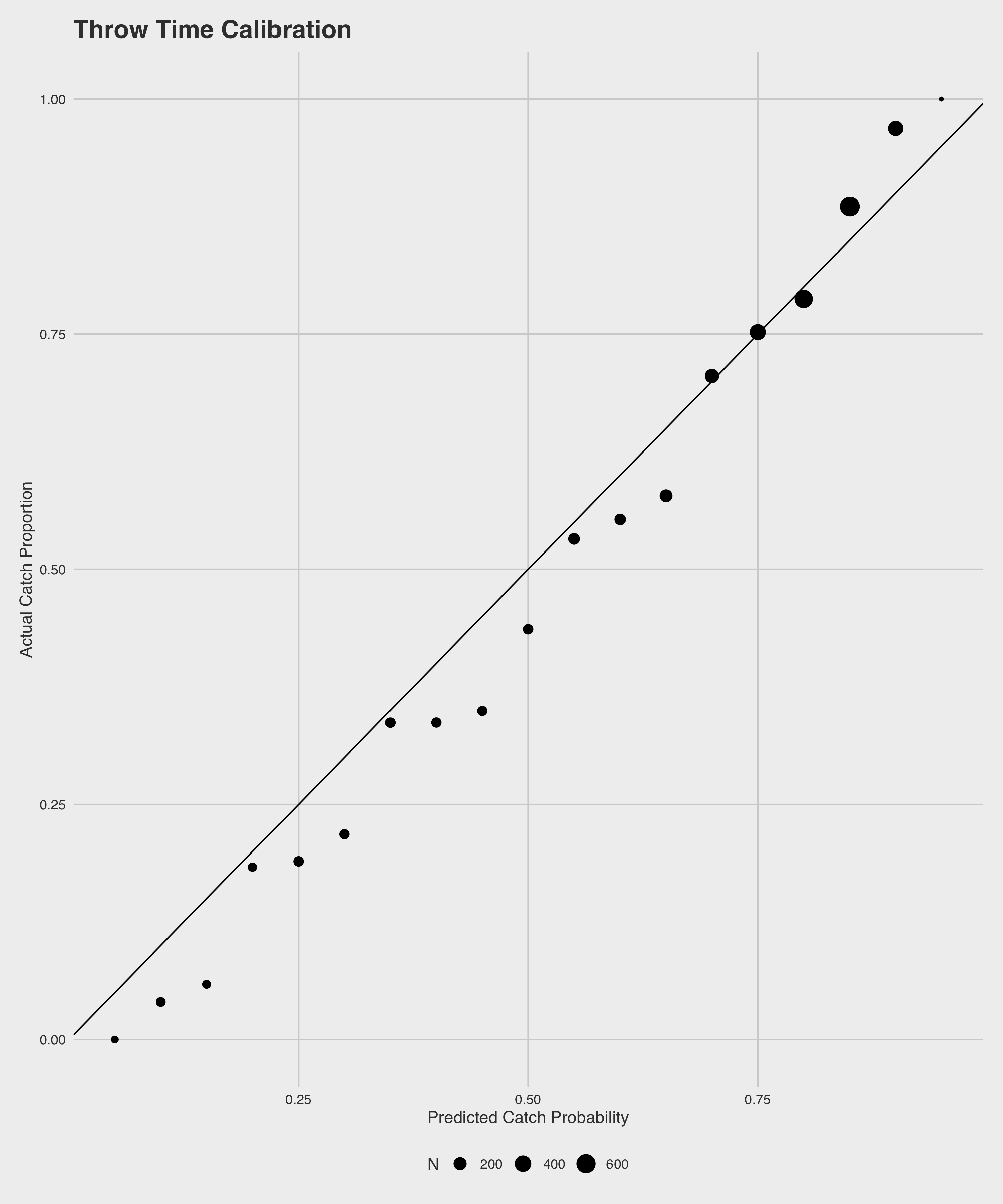
These two models both perform quite well, and far better than random chance. The throw model accurately predicts \(74\%\) of all passes, with strong precision (\(84\%\)) and recall (\(76\%\)), and an AUC of \(0.81\). As can be expected, our arrival model outperforms the throw model in all measures - accurately predicting \(78\%\) of all passes with a precision of \(88\%\), a recall of \(79\%\), and an AUC of \(.87\). All of these metrics were calculated on a held-out data set not used in model training. Below are plots of the calibration of the predictions of each of the models on the same held-out set.

cal_plot_arrival_model cal_plot_throw_model

We can do a few particularly interesting things with the predictions from these two models in tandem. Namely, we can use the two to calculate marginal effects of the play of the defensive backs. A simple example is as follows: For a given pass attempt, our throw model estimates that there is a \(80\%\) chance of a catch. By the time that pass arrives, however, our arrival model estimates instead that there is a \(50\%\) chance of a catch. Ultimately, the play results in a drop. In total, our defense can get credit for \(+.8\) drops, but we can break it down into \(+.3\) drops worth from closing on the receiver and \(+.5\) drops from breaking up the play, based on how the individual components differ. In other words, we subtract the probability of a catch at arrival time from the probability at throw time to get the credit for closing down the receiver, and we subtract the true outcome of the play from the probability of a catch at arrival time to get the credit for breaking up the pass.

The main challenge comes not from calculating the overall credit on the play, but from the distribution of credit among the defenders. In the previous example where we have to credit the defense with \(+.8\) drops added, who exactly on the defense do we give that credit to? There are a couple of heuristics that might make sense. One option would be to just split the credit up evenly among the defense, but this would be a bad heuristic because some defenders will have more of an impact on a pass being caught than others, and thus deserve more credit. We might also give all of the credit to the nearest defender, but that would be unfair to players who are within half a yard of the play and are also affecting its outcome but would get no credit under this heuristic. Ultimately, we opted to use the models to engineer the credit each player deserves by seeing how the catch probabilities would change if we magically removed them from the field, which we believe to be a better heuristic than the previous ones described. To implement this heuristic, we remove one defender from our data and re-run the predictions to see how big the magnitude of the change in catch probability is. The bigger the magnitude difference, the more credit that player gets. Then, we calculate the credit each defender gets with \(credit_{i} = \frac{min(d_{i}, 0)}{\sum_{i} min(d_{i}, 0)}\) where \(d_{i}\) is the catch probability without that player on the field minus the catch probability with him on the field. In other words, if one player gets \(75\%\) of the credit for a play and the play is worth \(+.8\) drops added, then that player gets \(.8 \cdot .75 = +.6\) drops of credit, and the remaining \(+.2\) drops are divvied up amongst the other defenders in the same fashion.

Target Probability

Our target model is based on comparing the probabilities that a receiver is targeted before the play begins and when the ball is thrown with the actual receiver targeted. We can use these probabilities to make estimates of how well the defender is covering (are receivers less likely to be thrown the ball because of the pre-throw work of a defensive back?) and how much respect they get from opposing offenses (do quarterbacks tend to make different decisions at throw time because of the defensive back?).

To determine the probability of a receiver being targeted before the play, we chose to take a naive approach. Each receiver on the field is assigned a “target rate” of \(\frac{targets}{\sqrt{plays}}\), which is then adjusted for the other receivers on the field and used as the only feature for a logit model. The idea of this rate was to construct a statistic that rewarded receivers for showing high target rates over a large sample but also gave receivers who play more often more credit.

The model for target probability at the time of throw was a tree booster similar to the two catch probability models. This model uses positional data, comparing the receiver position to the QB and the three closest defenders along with a variety of situational factors such as the distance to the first down line, time left, weather conditions, and how open that receiver is relative to others on the play to determine how likely that receiver is to be targeted.

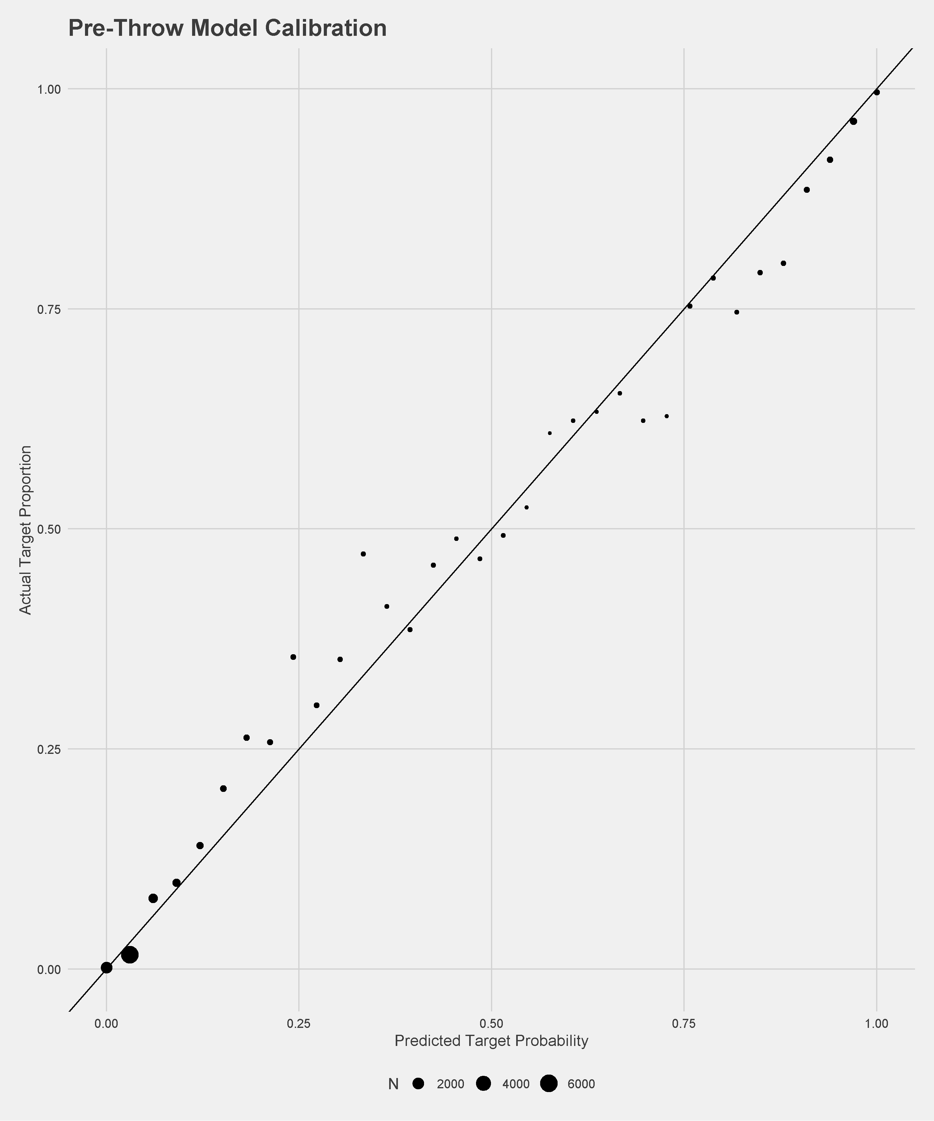
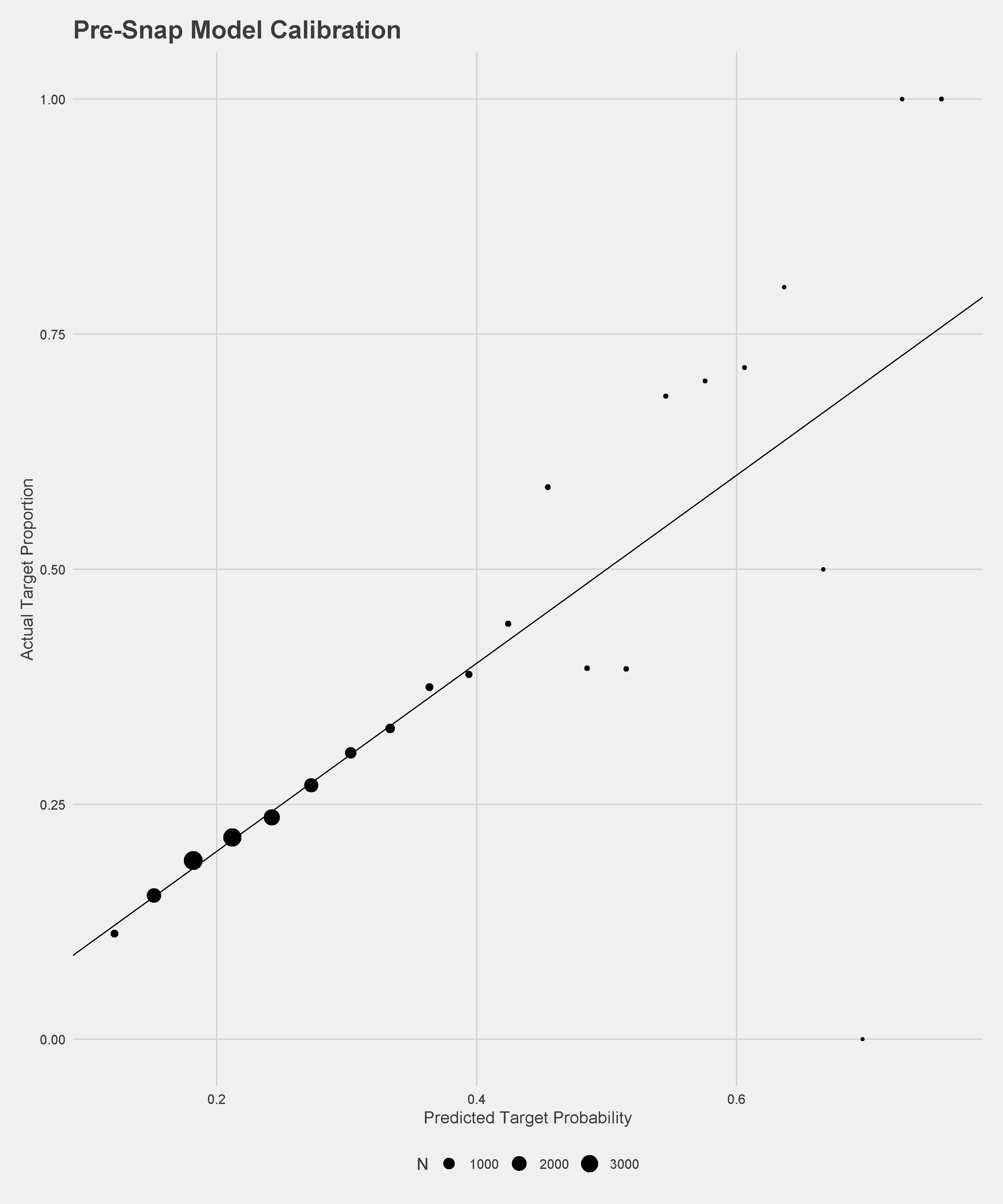
The pre-snap model, which by design only considers the players on the field for the offense, performs relatively well for the lack of information with an AUC of \(.59\) and is well-calibrated on a held-out dataset. The pre-throw model performs much better given the extra information, with \(89\%\) recall, \(94\%\) precision, and \(.94\) AUC. Calibration plots of the models on held-out data are below.

cal_plot_target_model_throw cal_plot_target_model_presnap

We can estimate how a defensive back is impacting the decisions made by the quarterback through two effects. The first, comparing the target probability before the play to the target probability at the time of the throw is meant to estimate how well the receiver is covered on the play. For example, consider a receiver with a target probability of \(20\%\) before the snap who ends up open enough to get a target probability of \(50\%\) when the ball is thrown. This difference is attributed to the closest defensive back who would be credited with \(-0.3\) coverage targets. If on the same play another receiver had a pre-snap target probability \(30\%\) but a target probability of \(0\%\) at throw time, the closest defensive back would be credited with \(+0.3\) coverage targets. The other effect attempts to measure how the quarterback is deterred from throwing when that particular defensive back is in the area of the receiver by comparing the probability of a target to the actual result. So if a certain receiver has a target probability of \(60\%\) at the time of the throw and isn’t targeted, the closest defender is credited with \(+0.6\) deterrence targets.

Results

Having produced these four models that gave us estimates of the influence of the defensive backs on a given play, we can accumulate the results over an entire season to produce an estimate of individual skill across the dimensions described by the models. As there is no straightforward way to measure the relative value of these skills, we chose to combine the individual skill percentiles for each defender as a measure of their overall skill. With that as the estimate, these are our top 15 pass-defending defensive backs in 2018:

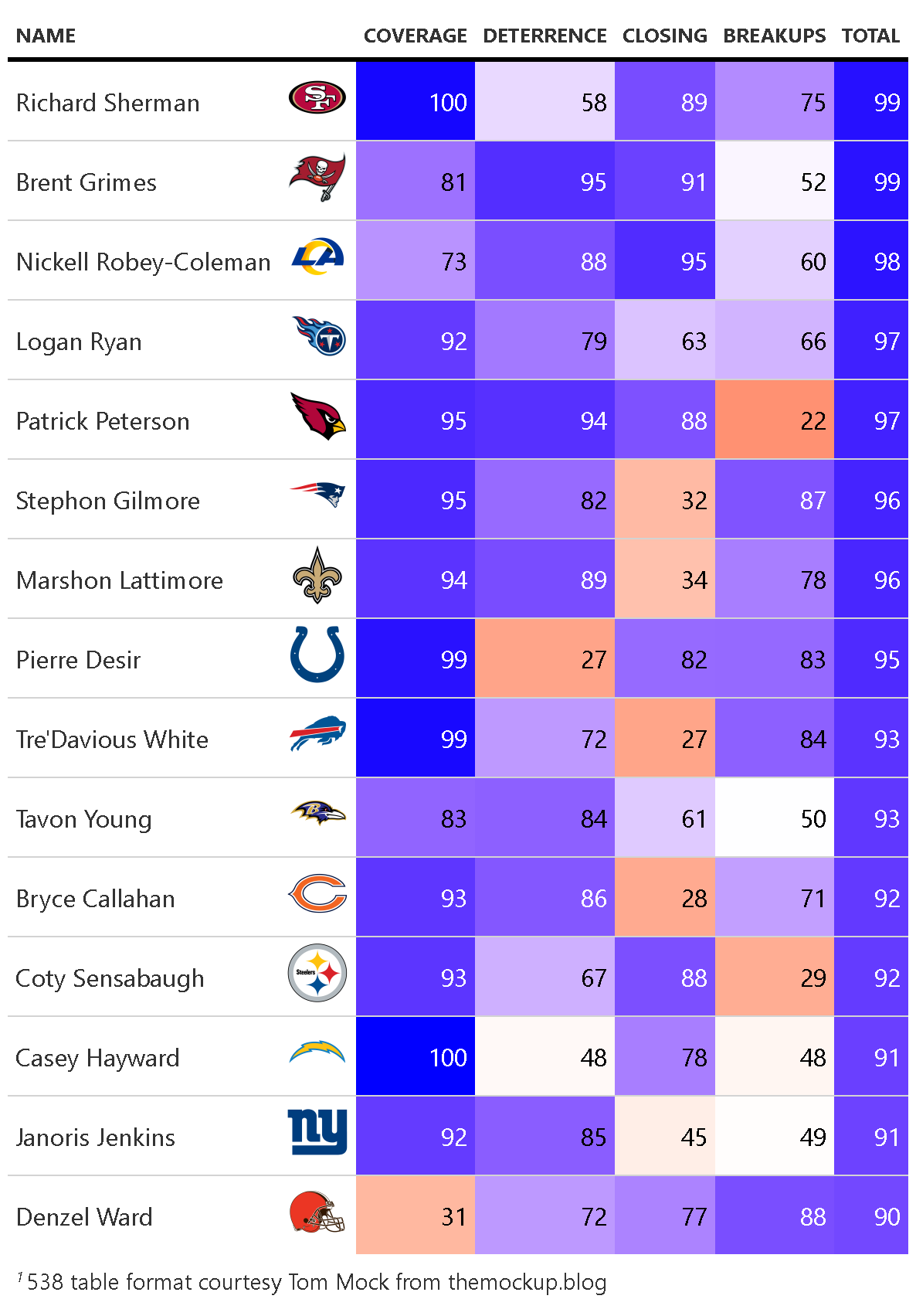
A full leaderboard of these can be found on our Shiny app in the Overall Rankings tab. To help display these results and a few other metrics (such as how difficult the defensive assignment was based on pre-snap target probability and actual separation from the receiver at throw time) we developed player cards for each qualifying defender. For example, this is our card for #1 defender Richard Sherman:

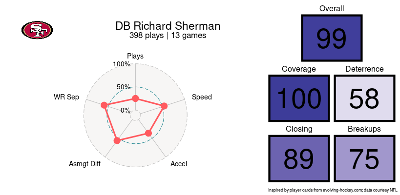
These cards can also be found on our Shiny app under Player Cards.

Further Work

There are several things that we didn’t consider or that would be interesting extensions of this project. Two clear ones are interceptions added and fumbles added, as those are hugely impactful football plays that can swing the outcomes of games. We also only considered raw changes in aggregating the player stats (i.e. targets prevented and drops added), but using EPA added instead would certainly be a better metric, since not all drops are created equal. In addition, it is not clear that a drop added is worth the same as a target deterred – an assumption we made – and EPA would help solve this problem too. It would also be interesting to test how similar our metrics are between seasons to confirm that our metrics are measuring the stable skill of a defender.

Appendix

All of our code is hosted in two Github repos: hjmbigdatabowl/bdb2021, which hosts our modeling code, and hjmbigdatabowl/bdb2021-shiny, which hosts the Shiny app.

There is extensive documentation for our code on our pkgdown site.

The Shiny app can be found here, which lets you explore our models, results, and player ratings.

Thoughts

First, a disclaimer for everything that follows: I’m extremely proud of what we submitted, and the work that we did. We spent hundreds of hours working on this project over about three months, which is an enormous undertaking for four people with other full-time commitments. Especially in the final weeks, I was spending well over ten hours a week working on this project, and probably closer to fifteen or twenty. All of that said, in the grand scheme of things, the 300 hours or so collective hours that we spent conceiving of and working on this project is nowhere near the amount of time and effort that could be poured into a project that a data science team of four was working on full-time for three months. Given more time, I believe there are significant ways in which we could have improved our final product.

Strengths

Communication and interpretability of the results. At the end of the day, when you work in a front office (as Hugh, John, and I know), you need coaches to believe what you’re telling them, and building a product that they can understand and explain is a major step in that direction. Overly complex or convoluted methodology will only get your work ignored, and I think that we did a particularly good job of building a product that is interpretable and useful.
Building a model that evaluates something useful. At the end of the day, I’m happy with the statistics we chose to put forward. In my view, barring special events like fumbles forced, tackling, and interceptions (all valuable things that should be worked on further to expand this project), the way that we evaluate defensive back performance by looking at what we view as the four major components – deterring passes by reputation, deterring passes with good positioning and coverage, closing down receivers, and breaking up passes – are the four most important skills for defensive backs in the NFL.
Divvying up credit in a clever way. I also think that the way we opted to divvy up the credit among the defenders in the two catch probability models was particularly clever, and not something that most teams would do. As we laid out in our submission, it doesn’t make sense to divvy credit evenly or give all credit to the nearest defender to the target, and I think that the approach that we took was both novel and easily defensible.

Weaknesses + Potential Improvements

Clearly, weighing each of the four components of defense that we measured equally is the wrong way to go. A better strategy would be to try to correlate them with defensive EPA or a similar stat and use the correlation coefficients / R-Squared values / MSEs / etc. to weigh the four components based on how strongly they predict EPA. The problem, though, is that we don’t have a defensive EPA, which means we’d need to model it. In addition, it’s unclear how to model a counterfactual. What I mean by that is that for a statistic like deterrence, we need to measure the EPA caused by a defender not being thrown at, which is an inherently difficult thing to model. So difficult, in fact, that I believe that the first NFL team to come up with a good way of doing this will have a Moneyball-esque leg up against the competition until other teams catch up (Ravens analysts, I’m looking at you).
There are other aspects of defensive performance that we’re not measuring. Two important categories are turnovers generated and YAC prevented. Both of these are hugely valuable for preventing points, and both are models that we didn’t have time to build.
Stability testing. We’re probably interested in how stable our metrics are across seasons. For example, does Stephon Gilmore being a 96 overall this year predict his rating next year at all? Since we only have one season of data, the answer is that we don’t know. This type of stability testing would be useful for predicting future performance, though.

General Thoughts

Again, I’m proud of what we’ve done here. In particular, spot-checking some of the numbers has been fascinating. There’s often very little correlation between metrics, which seems good, and often the correlations can be negative. The way to think about this, as my teammate Hugh eloquently put it, is that we should think about the negative correlations as being similar to \(ISO\) vs. \(K%\) in the MLB: A player who is fantastic in coverage and thus often deters throws necessarily will have fewer opportunities to break up passes, meaning he will see a lower score for closing, breakups, or both. We see this type of behavior with Gilmore, Peterson, Sherman, and more. It’s also been interesting to find that our models think the same corners are really good as the eye test does, which is an encouraging sign. Interestingly, though, some of our top-ranked defensive backs are players who don’t tend to make top lists, and some of our lowest-ranked ones (like Jason McCourty and Jalen Ramsey), do. This is reminiscent of the attitude changes about certain MLB players in the early 2010s as we began developing more advanced statistics to measure performance (i.e. Derek Jeter’s defense being terrible and Michael Bourn being sneakily good).

And with that, I’ve wrapped up my addendum to our submission. Feel free to reach out with any questions. My contact info is on my blog, my Github, my LinkedIn, etc. Thanks for reading!

Subscribe

Meta